



New: a desktop GUI (experimental). Set up, run and explore simulations in a window, with no script:
pip install "solprop[gui]", thensolprop-gui. See the desktop GUI and its section below.
Ultrafast nonlinear pulse propagation in Python — from few-cycle pulses in gas-filled hollow-core fibres to multimode solid-core fibres and free-space beams.
Everything, fast, with rigour. solprop aims to be one unified, highly accurate code for nonlinear pulse propagation, scaling from a laptop to a GPU cluster, with every model derived, cited and verified against analytic and independent references (About solprop).
It solves the unidirectional pulse propagation equation (UPPE) and the generalised nonlinear Schrödinger equation (GNLSE), for the full electric field or its envelope, in waveguides and in free space. Use it for soliton self-compression to sub-cycle pulses, resonant dispersive-wave emission into the vacuum and deep ultraviolet, supercontinuum generation, multimode and graded-index beam dynamics, filamentation, photoionisation and plasma, and Raman frequency combs.
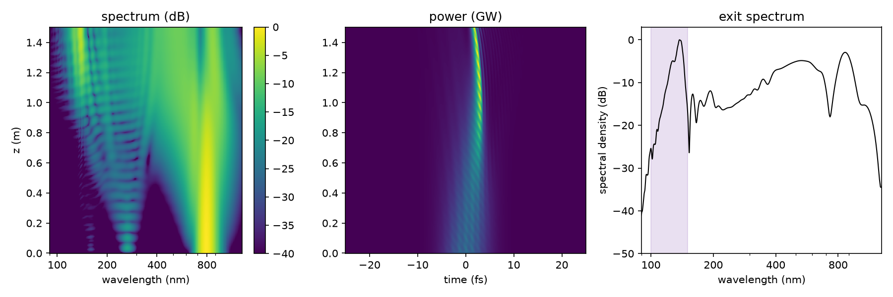
A 7.5 fs pulse at 800 nm self-compresses in a helium-filled capillary with a pressure gradient to vacuum and emits a resonant dispersive wave at 120–150 nm: spectral and temporal evolution along the 1.5 m fibre, and the exit spectrum. Four coupled modes, ionisation and plasma included; under ten seconds on a laptop.
from solprop.driver import prop_capillary
from solprop.plotting import prop_2d

run = prop_capillary(
    125e-6,  # core radius, m
    1.5,  # length, m
    "He",
    (0.8, 0.0),  # pressure gradient, bar: entrance to exit
    wavelength=800e-9,
    fwhm=7.5e-15,
    energy=275e-6,
    modes=4,  # the first four HE_1m modes
    trange=400e-15,
    wavelength_limits=(90e-9, 4e-6),
)
prop_2d(run, "wavelength")- Waveguides
- Gas-filled hollow capillaries, one or many modes, with tapers, pressure gradients and gas flow; a coherent wall that couples the modes and converts between them.
- Antiresonant hollow-core fibres (the Vincetti model); rectangular and planar guides; modes tabulated from any mode solver.
- Step-index and graded-index fibres with full vector modes, through a general modal route for any guide that supplies its own electric and magnetic fields — including guides that change along their length.
- Free space: beams in bulk gases and solids on radial, Cartesian and line grids, with the exact (non-paraxial) diffraction operator, absorbing spatial boundaries, and the Kerr, plasma and Raman responses of the guided routes: self-focusing, filamentation and ionisation in cells, jets and windows, and planar guides resolved across their width.
- Media and nonlinear responses: noble and molecular gases and their mixtures, glasses and metals, all from the curated material library optmat; Kerr and third-harmonic nonlinearity; photoionisation with optmat's atomic and molecular rate models, and plasma on field and envelope grids; rotational and vibrational Raman responses, scalar and vector; quantum shot noise; multi-colour inputs. An optional helium TDSE atomic response, for research, replaces Kerr and plasma by a microscopic atomic current; its native backend is not yet publicly available.
- Accurate numerics: two adaptive integrators, a low-call exponential Adams method (the default of capillary, radial and planar runs) and an embedded Runge–Kutta pair (the default of GNLSE, waveguide and Cartesian runs; the defaults), with the linear propagation integrated exactly, absorbing boundaries as rates, and every backend tested against a reference implementation within derived error bounds.
- Workflows: HDF5 output with resume, statistics along the fibre, parameter scans on
process pools and Slurm clusters, processing and plotting, soliton and dispersive-wave
design tools, and pulse compressors (Taylor phase, chirped mirrors, materials,
gratings and prisms). One import,
import solprop.sol as sol, sets up an interactive session.
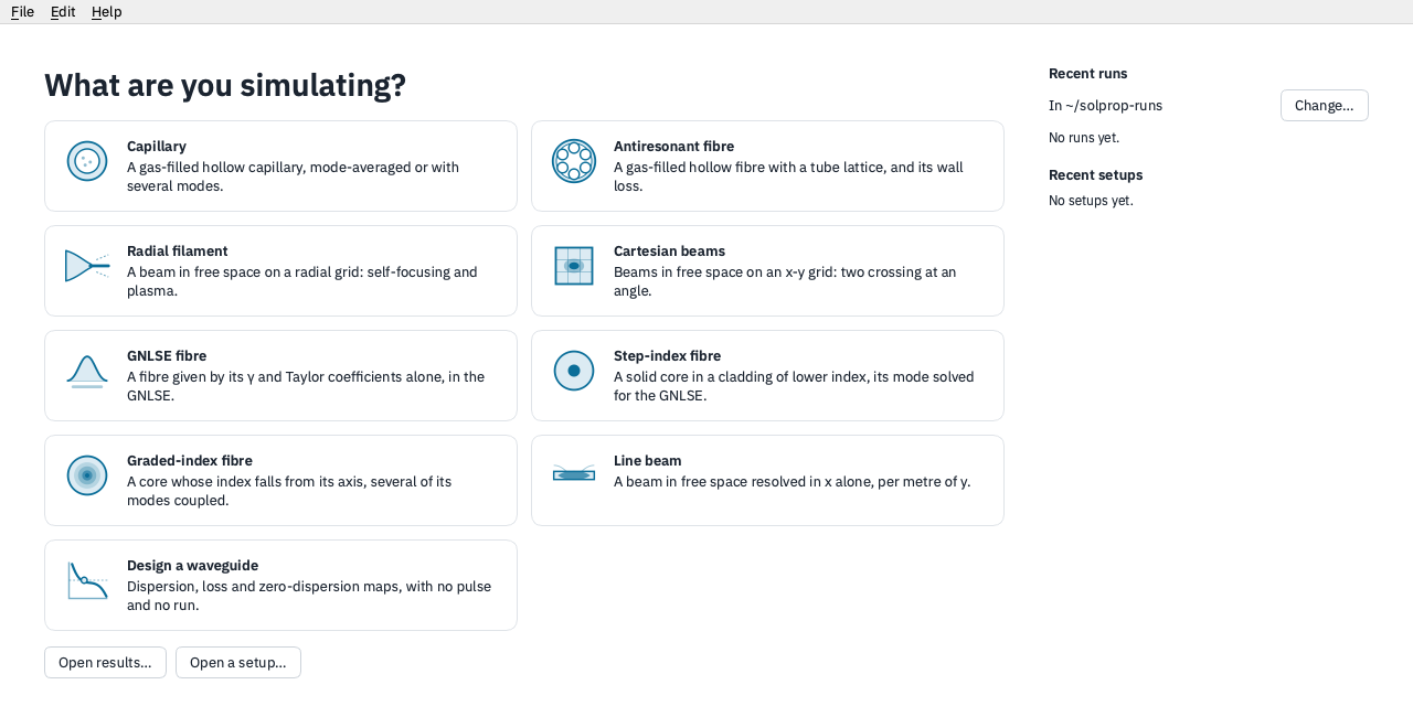
solprop now comes with an experimental desktop front end, solprop-gui, for setting up,
running and reading simulations without writing a line of Python:
pip install "solprop[gui]"
solprop-gui- Pick what you are simulating: gas-filled capillaries, antiresonant fibres, GNLSE, step-index and graded-index fibres, radial filaments, and Cartesian and line beams, each starting from a few chosen examples.
- One setup sheet, in physics terms: core radius, gas and pressure, pulse wavelength, duration and energy, checked as you type, with the numbers solprop computes for it (soliton order, zero-dispersion wavelength, fission length, P/Pcr) and a preview plot. Type a target into one of those numbers and solprop solves for the pressure or energy that gives it.
- Watch it run: the spectrum and the pulse grow along the fibre as it goes; stop it and resume it.
- Explore the results at any point along the propagation: maps, spectra, pulses,
spectrograms, energy, peak power and electron density along z, with zoom, readouts, widths at half
maximum, and publication figures drawn by
solprop.plotting. - Scan and design: run a grid over any parameters and open any point as a setup, or explore a waveguide's dispersion, loss and phase matching with no pulse at all.
- Never a dead end: every setup saves as a recipe or as the Python script that builds it, and every solprop results file opens in the window.
Its interface may still change between releases. The desktop GUI chapter of the user guide walks through it; the window's Help menu opens the same pages offline.
solprop-native, built from
native/ in this repository, is
the backend solprop runs on: C++ kernels built with
Kokkos, using OpenMP, FFTW and a vendor BLAS on multi-core CPUs, or
CUDA and HIP on NVIDIA and AMD GPUs. It is a required dependency, so pip install solprop
installs it and solprop uses it automatically; your scripts do not change.
numpy_ref, the plain NumPy backend that native is tested against, is the numerical
reference. It is unthreaded and roughly 6 to 40 times slower than threaded native, so it
is for checking a result and for the few supported features native does not run yet, the
TDSE response among them
(which backend to use). See
The native backend and
Performance tuning.
solprop needs Python 3.14 (3.15 is not yet supported: some dependencies have no wheels for it) and runs on Linux, macOS and Windows, wherever its native backend installs:
pip install solpropThis installs a precompiled wheel of the native backend, with no extra, on macOS on Apple
silicon (osx-arm64), Linux on x86-64 (linux-64), Linux on aarch64 (linux-aarch64), Windows
on x86-64 (win-64) and Windows on Arm (win-arm64). On any other platform the installer
reports that it found no matching distribution:
Installation explains that error and how to
report the platform, and covers environment checks and a first run. For GPUs, build the
native backend from source (below). Then run solprop calibrate once, to fit the native
backend's threads, waiting and transform plans to the machine
(Calibrating solprop to your machine).
Both packages build from one clone of the repository:
git clone https://github.com/LupoLab/solprop.git
cd solprop
pip install . ./native          # solprop and the native backend, for this machine's CPU
The native build needs a C++20 compiler, CMake, FFTW and, for speed, a BLAS. A GPU build (NVIDIA with CUDA, AMD with HIP, on Linux) is always compiled from source, with the device enabled through CMake options. Building the native backend gives the requirements, the commands for Linux, macOS, CUDA and HIP, and every build option. To work on solprop itself, see Contributing.
The manual is at solprop.readthedocs.io:
- Introduction — installation, capabilities, spatial descriptions, and first propagation calculations.
- User guide — simulation setup, waveguides and free space, materials and nonlinear responses, numerical methods, results, workflows, and performance, including the detailed equations and approximation limits.
- Examples — introductory lessons, focused demonstrations, and full worked simulations, organised by what they teach.
- Developer’s guide — contributing, architecture, implementation contracts, testing, tooling, proposals, and project history.
- API — the complete reference for functions, classes, and modules.
Users of solprop's predecessor, Luna.jl, can start with noteworthy differences from Luna.
solprop continues more than two decades of pulse-propagation codes by John Travers and colleagues, most recently Luna.jl; About solprop tells the story. solprop itself is developed almost entirely by AI coding agents under the lead developer's direction, within a strict harness of derivations, reference comparisons, convergence checks and complete test coverage; the same page explains how, and what that means for users. The code is free software under the GNU General Public License, version 3 or (at your option) any later version, and the documentation is under CC BY 4.0. Contributions are welcome: see CONTRIBUTING.md. If you use solprop in published work, please cite its Zenodo record, doi:10.5281/zenodo.23854248, and the version you used.